Spatial Datasets
Spatial transcriptomic datasets can be visualized and analyzed in rakaia. The preprocessing steps for spatial datasets are slightly different from antibody-based imaging datasets, and will also vary slightly across different technologies.
Required format
All spatial datasets that contain marker expression need to be pre-processed and imported into rakaia as an Anndata object; crucially, this file putput must have the file extension .h5ad to be read into rakaia. More specifically, the Anndata object must have a spatial array in the obsm slot that contains both the x and y coordinates for each spatial measurement, whether it corresponds to a cell, spot, etc. Libraries such as scanpy and squidpy are Python libraries that have provide readers for raw spatial data into this format. These libraries will be referenced in the article below.
Spot-based assays: 10X Visium V1, V2
Spot-based spatial technologies such as the 10X Visium Spatial Gene Expression profile transcript counts summarized at the spot level. The Visium technology is capable of profiling tens of thousands of markers per spot, providing comprehensive spatial context of the transcriptome.
Raw Visium data (from the space ranger standard directory output as described here) should be read using either read_visium function from either scanpy or squidpy. Below is a minimal example showing how the data can be preprocessed and exported into a compatible file format:
from scanpy import read_visium
import os

# specify the input directory with the outs subdir
input_dir = "/path_to_visium_raw/outs/"

adata = read_visium(input_dir)
adata.var_names_make_unique()

# specify the output file as an anndata object
out_anndata = "/output_dir/visium.h5ad"
adata.write_h5ad(out_anndata)
The output h5ad Visium file should typically not be larger than 200-300mb. If the size signficantly exceeds this range (1-2 GB or larger), then it is likely that the user has cached a full-sized WSI (i.e. H & E) in the file. Caching these large images will result in significant performance slowdowns in rakaia. To avoid this, users should ensure that the uns slot in the object is cleared of any fields except the required scalefactors slot:
adata.uns = {'spatial': {str(list(adata.uns['spatial'].keys())[0]): {
           'scalefactors': adata.uns[
               'spatial'][list(adata.uns['spatial'].keys())[0]]['scalefactors']}}}
This retains the scale factors required for Visium to render in rakaia, while removing any additional slot caches that rakaia does not use.
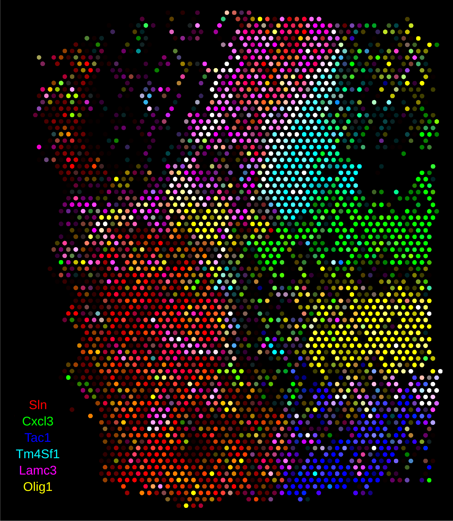
When the Anndata object is read into rakaia, the spot size and region dimension will automatically be computed from the spatial coordinates and scale factors:
Non-spot based assays
Non spot-based assays behave differently in rakaia as the user has more flexibility over the visualization parameters. Specifically, this means that the user may specify a unique visualization size for the data in the image, which isn't supported with spot-based assays because the spot scaling factors are computed automatically from the input data.
Binned expression assays: 10x Visium HD
The HD version of 10X Visium differs slightly from the spot-based technology used in either V1 or V2. Instead of using circular spots that have gaps among them, HD offers tiled, barcoded squares without gaps, as described here. This results in data that can be binned at summarized at three different micron resolutions: 2, 8, and 16.
Currently, the only supported reader in Python for HD datasets is the spatialdata HD reader. The reader generates aggregate expression profiles for each micron resolution, and each of these profiles can be exported as an Anndata file for visualization in rakaia. This example notebook here shows an example of how to export these binned profiles. each bin can then be imported into rakaia as a separate ROI with the same set of marker genes, but with different dimensions and resolution.
10X Xenium In-situ Expression
The 10X Xenium platform differs slightly from the assays above as it profiles in-situ transcript profiles, and also supports segmentation and the overlay of object masks. The notebook example here provides a complete example of reading the data into a spatialdata object and exporting both the expression Anndata object as well as the separate cell segmentation mask as a tiff.
Setting marker sizes for visualization (non spot-based)
The non spot-base technologies above support custom user marker sizes in rakaia. This means that the marker can be visually enlarged or minimized down to a default size of 1 pixel in the viewer. This allows the expression to appear more granular/minimal or more extensive/uniform throughout the ROI as the user desires.
Below are some recommended marker sizes for the different technologies listed above. The marker size can be changed under Additional application settings -> Appearance -> Custom spatial marker radius.
-
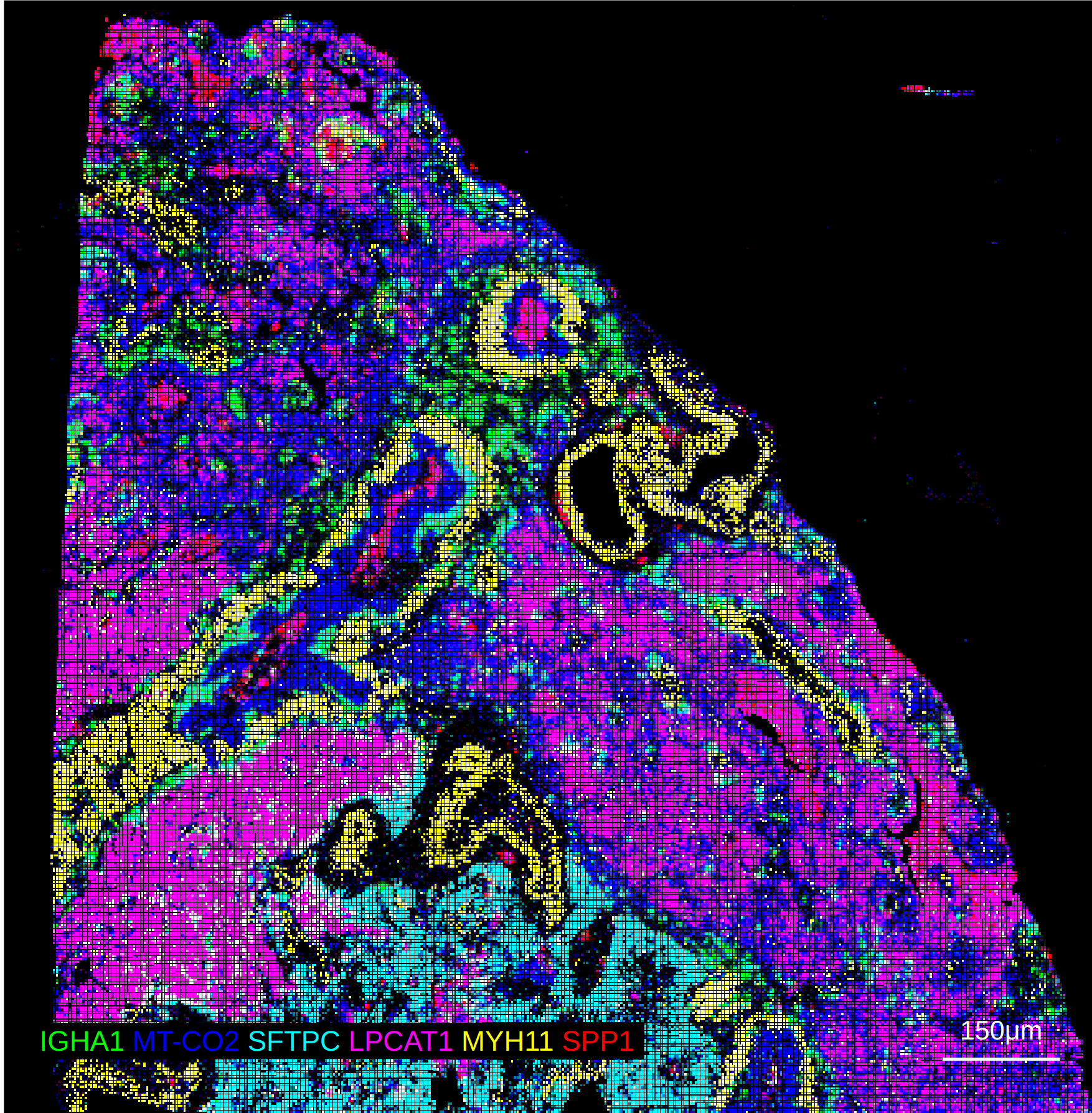
10X Visium HD: 2-3. A marker size of 2 will generaly reveal pixel gaps between areas of expression, with 3 removing those gaps and providing a more uniform, albeit maybe slightly blurred, expression visualization. Generally, marker sizes of 4 of greater will cause expression to overlap erroneously.
-
10X Visium: 2-4. The marker size should be set based on the presence of an overlaid segmentation mask. Without using a segmentation mask, larger marker sizes up to 4 will make the expression more visually appealing at a global resolution, but could result in markers that "spill" out of the segmentation mask. When using a mask, values of 2-3 allow the marker to appear in the centroid of the cell mask while also allowing the expression to appear at the global resolution.
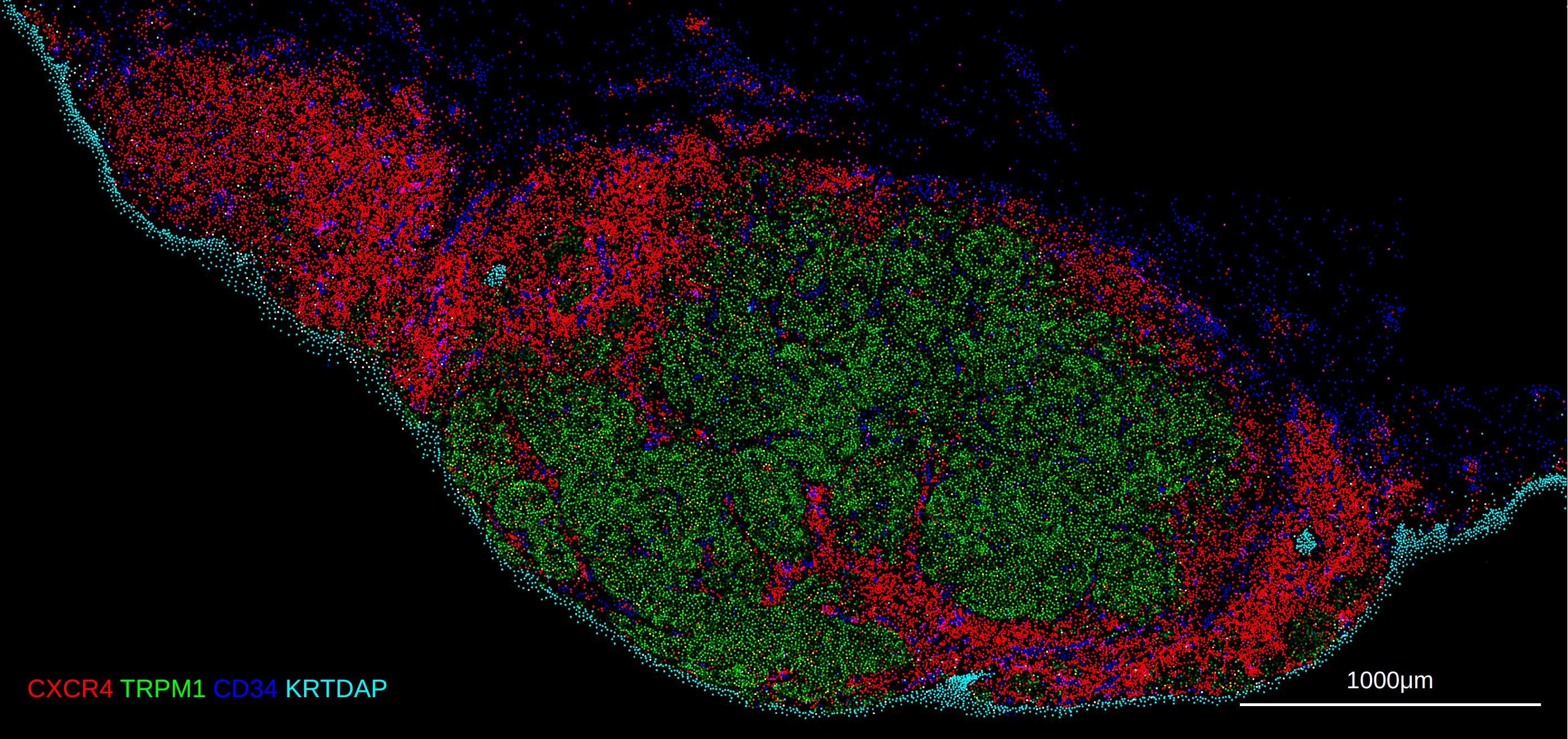
Setting a larger marker size increases the possibility of seeing overlapping or fragmented expression spots in 10X Xenium assays. This is particularly noticeable in dense tissue where cells may be close together, or areas where it is difficult to clearly segment cell boundaries. Additionally, filtering spotrs using a lower bound may cause visual fragmentation of spots, as a portion of the overlapping expression point may be filtered out. In these instances, users may want to reduce the marker size incrementally until the markers no longer touch/overlap.
Other spatial datasets
Additional spatial technologies may be inherently supported in rakaia provided that they follow the input data format as described above (minimally, that spatial coordinates for pixel locations are provided in spatial array in the obs slot).
Additional examples of spatial datasets that can be rendered in rakaia include the following from the squidpy spatial technology tutorials:
-
Vizgen: https://squidpy.readthedocs.io/en/stable/notebooks/tutorials/tutorial_vizgen.html
-
4i: https://squidpy.readthedocs.io/en/stable/notebooks/tutorials/tutorial_fouri.html
-
Slide-seq: https://squidpy.readthedocs.io/en/stable/notebooks/tutorials/tutorial_slideseqv2.html
For all tutorial datasets above, the data are imported and anlayzed in Anndata format, consistent with the required format for rakaia. The adata object referenced in the tutorials can be exported as files with the .h5ad format.
rakaia features not available to spatial datasets
Spatial datasets have orders of magnitude more variables and markers than IMC datasets (tens of thousands of markers as opposed to 40-50 antibodies), so the lazy loading features behave differently for these technologies. This means that certain features that can be applied to an entire ROI for IMC cannot be used for spatial analysis due to memory and time constraints in processing all dataset markers:
- The channel/marker tile gallery is not supported for as generating a thumbnail preview for thousands of markers would be prohibitively time-consuming
- Both marker correlation and in-app marker quantification can be performed only on markers that are in the current canvas, as these are the only variables that have been loaded into memory at a given point in analysis